Notes:
- this post is about how transformers are implemented, not why they’re implemented the way they are.
- This post assumes the reader understands what is meant by training a model, parameters and hyperparameters, dense layers, and so on.
- We’ll be using jax and flax for this implementation.
Overview
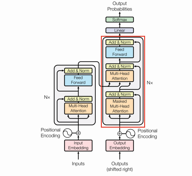
The following is the transformer architecture diagram taken from the original paper. We’ll be referring back to it often in this post.
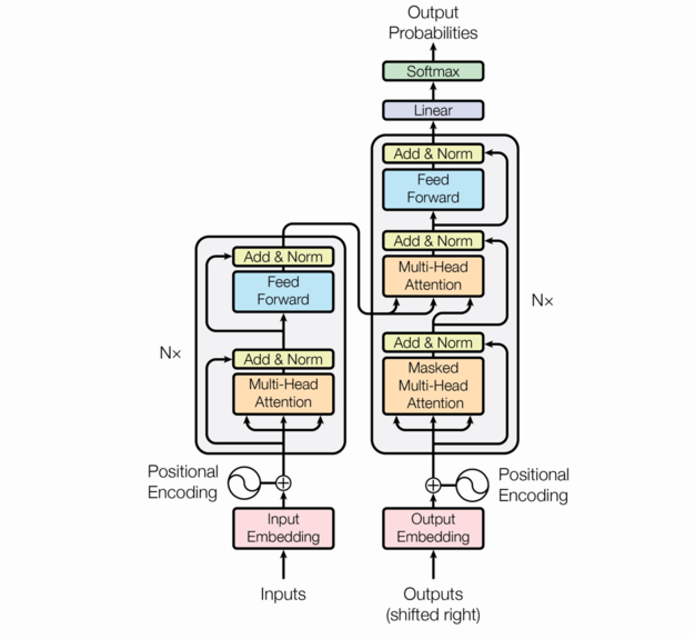
At a high level, the transformer is an encoder-decoder model; it takes a sequence of tokens from a source (e.g. English words) and learns to translate that into a destination sequence (e.g. French words). There are three flavors of transformers: encoder/decoder, encoder-only, and decoder-only. This post will focus on encoder/decoder transformers.
from typing import Callable, Sequence

import chex
import jax.numpy as jnp
import jax.random as jran
import jax.tree_util
import optax
from flax import linen as nn
from IPython.display import display
from tqdm.auto import tqdm

key = jran.PRNGKey(0)
Input (output) embeddings
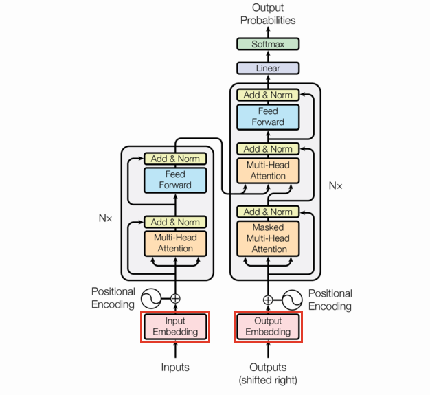
As we said before, the transformer model is a sequence to sequence model. Natural language lends itself to many possible sequence definitions (words, characters, bigrams, etc.), so strictly speaking we need to define a tokenizer before we even get to the Embeddings.
Tokenization
The tokenizer takes something like natural language and returns a sequence (typically of unique natural numbers – IDs). We’ll tokenize each character "a" through "z" along with the requisite start and pad tokens (represented by "<start>" and "<pad>" respectively – to be explained later). So our tokens are ["a", "b", "c", ..., "z", "<start>", "<pad>"], and our tokenizer maps those to [0, 1, 2, ..., 25, 26, 27].
vocab = {chr(97 + i): i for i in range(26)}
vocab['<start>'] = len(vocab)
vocab['<pad>'] = len(vocab)
One reason transformers really took off (in their early days) was that you could easily train them in batches without the recurrence required of something like RNNs. In order to do that, we need to arrange our sequences into a batch. But what if the sequences are of different lengths? For that we use numpy’s pad function: we fill in the empty spots at the end of the shorter sequences with our '<pad>' token so that we can ignore these in our loss.
def str2ids(txt, vocab=vocab):
    return jnp.array([vocab[x] for x in txt])


def strs2ids(*txts, vocab=vocab):
    ids = [str2ids(x, vocab=vocab) for x in txts]
    maxlen = max([len(x) for x in ids])
    return jnp.stack([jnp.pad(jnp.array(x), pad_width=(0, maxlen - len(x)),
                              mode='constant', constant_values=vocab['<pad>'])
                      for x in ids])

def ids2str(ids, vocab=vocab):
    x = [list(vocab)[x] for x in ids]
    x = [y if y != '<pad>' else '~' for y in x]
    return ''.join(x).rstrip('~')

def ids2strs(ids, vocab=vocab):
    return [ids2str(x, vocab=vocab) for x in ids]

seq = ['hey', 'there', 'ma', 'dood']
assert ids2strs(strs2ids(*seq)) == seq
display(strs2ids(*seq))
del seq
Array([[ 7,  4, 24, 27, 27],
       [19,  7,  4, 17,  4],
       [12,  0, 27, 27, 27],
       [ 3, 14, 14,  3, 27]], dtype=int32)
Notice how 27 appears in that matrix – 27 is our "<pad>" token.
Embedding
After tokenization, the Input Embedding is the start of the data flow. An embedding is a mapping from a discrete set with cardinality $N$ to a subset of $\mathbb{R}^d$ where $d\ll N$. This is generally done in such a way that a the topology is preserved. It can be broken down into two parts:
- An $N\times d$ parameter matrix (also called a rank-2 tensor).
- An association between each element of our discrete set and a row in that matrix.
The second part comes naturally from our vocabulary definition (we can map each token to the integer the vocabulary maps it to).
The first part is already implemented in flax. We instantiate an example nn.Embed layer below with $N=28$ and $d=2$ (using the notation above). You can see that the embedding layer only has one parameter, 'embedding', which is a $N\times d$ matrix. $d$ is called the embedding dimension.
model = nn.Embed(len(vocab), 2)
params = model.init(key, jnp.array([1]))
jax.tree_util.tree_map(jnp.shape, params)
{'params': {'embedding': (28, 2)}}
If we get some embeddings, we see that the model is doing exactly what we said it would do (it’s just grabbing the $i^\text{th}$ row of the matrix).
model.apply(params, str2ids('abc'))
Array([[ 0.35985   , -0.75417924],
       [-1.206328  ,  0.7793859 ],
       [ 0.11096746, -1.0079818 ]], dtype=float32)
params['params']['embedding'][0:3]
Array([[ 0.35985   , -0.75417924],
       [-1.206328  ,  0.7793859 ],
       [ 0.11096746, -1.0079818 ]], dtype=float32)
These weights get tuned thereby “learning” an $d$-dimensional embedding for each token.
Positional encoding
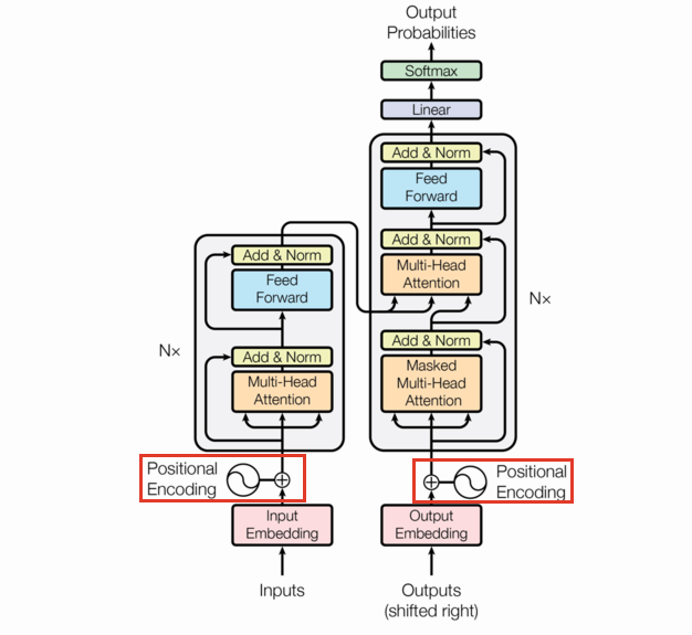
The positional encoding is the same size as a single observation fed to the model and added to each observation in the batch. We use the same function as they used in the original paper. Let $X\in\mathbb{R}^{s\times d}$ where $s$ is the max sequence length, and $d$ is the embedding dimension.
\[f(X_{i,j}) = \begin{cases} \sin\left(i/\left(10000^{j/d}\right)\right) & \text{if } j\equiv 0\pmod{2} \\ \cos\left(i/\left(10000^{(j-1)/d}\right)\right) & \text{if } j\equiv 1\pmod{2} \end{cases}\]def sin_pos_enc(sequence_length, embed_dim):
"""create sin/cos positional encodings
Parameters
==========
sequence_length : int
The max length of the input sequences for this model
embed_dim : int
the embedding dimension
Returns
=======
a matrix of shape: (sequence_length, embed_dim)
"""
chex.assert_is_divisible(embed_dim, 2)
X = jnp.expand_dims(jnp.arange(sequence_length), 1) / \
jnp.power(10000, jnp.arange(embed_dim, step=2) / embed_dim)
out = jnp.empty((sequence_length, embed_dim))
out = out.at[:, 0::2].set(jnp.sin(X))
out = out.at[:, 1::2].set(jnp.cos(X))
return out
sin_pos_enc(5, 2)
Array([[ 0.        ,  1.        ],
       [ 0.841471  ,  0.5403023 ],
       [ 0.9092974 , -0.41614684],
       [ 0.14112002, -0.9899925 ],
       [-0.7568025 , -0.6536436 ]], dtype=float32)
We’ll come back to this later.
Multi-Head Attention
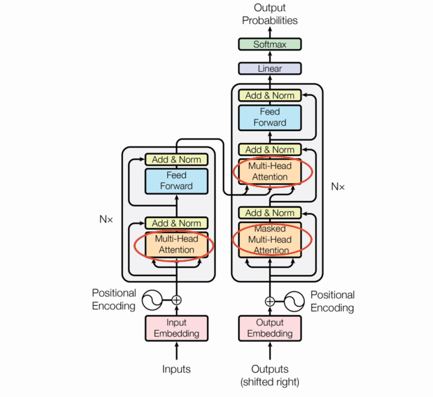
Transformers are built around the Multi-Head Attention you see in the picture, but MHA is itself built on attention. Attention is just a function that takes 3 matrix arguments (query, key, and value) and aggregates them to a vector. There are a few forms of attention but we’ll focus on the one used in the seminal paper: scaled dot product attention.
Scaled dot product attention
Let $Q\in\mathbb{R}^{n\times d},K\in\mathbb{R}^{m\times d},V\in\mathbb{R}^{m\times v}$ be the query, key, and value. Basically we just need the shapes to be fit for the matrix multiplication below. A good reference for this is d2l.ai.
\[\text{softmax}\left(\frac{QK^T}{\sqrt{d}}\right)V\in\mathbb{R}^{n\times v}\]The $\text{softmax}\left(\frac{QK^T}{\sqrt{d}}\right)$ part is called the attention weights.
It’s worthwhile to note that there are no learnable weights in this formula.
This formula is deceptive in 2 ways:
- The softmax is often masked
- There’s generally some dropout on the attention weights
Masked softmax
Let $X\in\mathbb{R}^k$ a vector, then $\text{softmax}(X)\in\mathbb{R}^k$.
\[\text{softmax}(X)_i = \frac{e^{X_i}}{\sum_{j=0}^{k-1}e^{X_j}}\]It’s just normalization with a monotonic function applied, meaning the relative ranking of the elements of $X$ aren’t changed. For more on this, see this post.
For masked softmax, we’ll be taking the approximate approach. Because of the sum in the denominator and the exponentiation, it’s unwise to mask with 0 ($e^0 = 1$). Instead we’ll mask with a very large negative number before we exponentiate so that the result is close to 0 ($e^{-\infty} \approx 0$).
def masked_softmax(args, mask):
    if mask is not None:
        args = args + (mask.astype(args.dtype) * -10_000.0)
    return nn.softmax(args)

def dot_prod_attn(q, k, v, dropout=lambda x: x, mask=None):
    # NxD @ DxM => NxM
    # (B[, H], N, M)
    attn_scores = q @ k.swapaxes(-2, -1) / jnp.sqrt(q.shape[-1])
    attn_weights = masked_softmax(attn_scores, mask)
    # (B[, H], N, D)
    out = dropout(attn_weights) @ v
    return out, attn_weights

# these are 13 batches of Q, K, V matrices arranged into rank 3 tensors
Q = jran.normal(jran.fold_in(key, 0), (13, 3, 7))
K = jran.normal(jran.fold_in(key, 1), (13, 5, 7))
V = jran.normal(jran.fold_in(key, 2), (13, 5, 11))

print(jax.tree_map(jnp.shape, dot_prod_attn(Q, K, V)))
del Q, K, V
((13, 3, 11), (13, 3, 5))
Multihead Attention
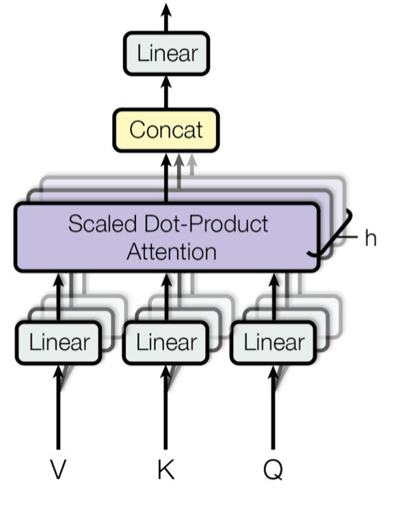
Multi-head attention involves stacking a collection of attention “heads” and adding some learned weights in the mix. As such, we’ll start with attention heads and progress to multi-head attention.
At a high level, mutli-head attention is a bunch of stacked attention layers. But given that there are no learnable weights in the attention heads (they query, key, and values are all arguments), each would yield the same result – not so useful. So instead, we train a linear layer per attention head, and then concatenate the results.
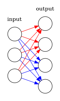
One linear vs stacked linears
Many implementations use one linear layer and reshape the output rather than storing a collection of linear models. At first this might not seem kosher, but it is. The picture below shows how 2 attention heads (red and blue) can be trained with one linear model.
class MultiHeadAttention(nn.Module):
    n_heads: int
    size_per_head: int
    attn_dropout: float
    fc_dropout: float
    attn_fn: Callable = dot_prod_attn

    @nn.compact
    def __call__(self, q, k, v, mask=None, *, training=False):
        "expected shape: Batch, [N|M], Dim"
        B, N, D = q.shape
        _, M, _ = k.shape

        def qkv_layer(x, name):
            x = nn.Dense(self.n_heads * self.size_per_head, name=name)(x)
            x = x.reshape((B, -1, self.n_heads, self.size_per_head)).swapaxes(1, 2)
            return x
        # BxNxD => BxHxNxP
        q = qkv_layer(q, 'query_linear')
        # BxMxD => BxHxMxP
        k = qkv_layer(k, 'key_linear')
        # BxMxD => BxHxMxP
        v = qkv_layer(v, 'value_linear')
        if mask is not None:
            # accounting for reshape in qkv_layer
            # B[xN]xN   => Bx1[xN]xN
            mask = jnp.expand_dims(mask, 1)
            if mask.ndim < q.ndim:
                # softmax is applied to dim -1
                # Bx1xN => Bx1x1xN
                mask = jnp.expand_dims(mask, -2)
        attn_do = nn.Dropout(self.attn_dropout, deterministic=not training, name='attn_dropout')
        out, attn_weights = self.attn_fn(q, k, v, attn_do, mask=mask)
        # uncomment to keep attention weights in state
        # self.sow('intermediates', 'weights', attn_weights)
        out = out.swapaxes(1, 2).reshape((B, N, -1))
        out = nn.Dense(D, name='output_linear')(out)
        out = nn.Dropout(self.fc_dropout, deterministic=not training, name='fc_dropout')(out)
        return out
As we all know at this point, these models can get quite big. It turns out, transformers are just naturally large models. Below we show that even a pathalogically simple MultiHeadAttention layer has 63 parameters!
batch_size = 2
sequence_length = 5
embed_dim = 3
n_heads = 2
size_per_head = 2

X = jnp.arange(batch_size * sequence_length * embed_dim)
X = X.reshape((batch_size, sequence_length, embed_dim))

mdl = MultiHeadAttention(n_heads, size_per_head, attn_dropout=0.2, fc_dropout=0.3)
params = mdl.init(key, X, X, X, mask=(jnp.max(X, axis=-1) < 0.8).astype(jnp.float32))

nn.tabulate(mdl, key, console_kwargs={'force_jupyter': True})(X, X, X)
del batch_size, sequence_length, embed_dim, n_heads, size_per_head, X, mdl
                                    MultiHeadAttention Summary
┏━━━━━━━━━━━━━━━┳━━━━━━━━━━━━━━━━━━━━┳━━━━━━━━━━━━━━━━━━┳━━━━━━━━━━━━━━━━━━┳━━━━━━━━━━━━━━━━━━━━━━┓
┃ path          ┃ module             ┃ inputs           ┃ outputs          ┃ params               ┃
┡━━━━━━━━━━━━━━━╇━━━━━━━━━━━━━━━━━━━━╇━━━━━━━━━━━━━━━━━━╇━━━━━━━━━━━━━━━━━━╇━━━━━━━━━━━━━━━━━━━━━━┩
│               │ MultiHeadAttention │ - int32[2,5,3]   │ float32[2,5,3]   │                      │
│               │                    │ - int32[2,5,3]   │                  │                      │
│               │                    │ - int32[2,5,3]   │                  │                      │
├───────────────┼────────────────────┼──────────────────┼──────────────────┼──────────────────────┤
│ query_linear  │ Dense              │ int32[2,5,3]     │ float32[2,5,4]   │ bias: float32[4]     │
│               │                    │                  │                  │ kernel: float32[3,4] │
│               │                    │                  │                  │                      │
│               │                    │                  │                  │ 16 (64 B)            │
├───────────────┼────────────────────┼──────────────────┼──────────────────┼──────────────────────┤
│ key_linear    │ Dense              │ int32[2,5,3]     │ float32[2,5,4]   │ bias: float32[4]     │
│               │                    │                  │                  │ kernel: float32[3,4] │
│               │                    │                  │                  │                      │
│               │                    │                  │                  │ 16 (64 B)            │
├───────────────┼────────────────────┼──────────────────┼──────────────────┼──────────────────────┤
│ value_linear  │ Dense              │ int32[2,5,3]     │ float32[2,5,4]   │ bias: float32[4]     │
│               │                    │                  │                  │ kernel: float32[3,4] │
│               │                    │                  │                  │                      │
│               │                    │                  │                  │ 16 (64 B)            │
├───────────────┼────────────────────┼──────────────────┼──────────────────┼──────────────────────┤
│ attn_dropout  │ Dropout            │ float32[2,2,5,5] │ float32[2,2,5,5] │                      │
├───────────────┼────────────────────┼──────────────────┼──────────────────┼──────────────────────┤
│ output_linear │ Dense              │ float32[2,5,4]   │ float32[2,5,3]   │ bias: float32[3]     │
│               │                    │                  │                  │ kernel: float32[4,3] │
│               │                    │                  │                  │                      │
│               │                    │                  │                  │ 15 (60 B)            │
├───────────────┼────────────────────┼──────────────────┼──────────────────┼──────────────────────┤
│ fc_dropout    │ Dropout            │ float32[2,5,3]   │ float32[2,5,3]   │                      │
├───────────────┼────────────────────┼──────────────────┼──────────────────┼──────────────────────┤
│               │                    │                  │            Total │ 63 (252 B)           │
└───────────────┴────────────────────┴──────────────────┴──────────────────┴──────────────────────┘

                                   Total Parameters: 63 (252 B)
We’re going to want to see keep track of how many parameters we have as we go, and looking at a giant table is just not very efficient. To that end, let’s write a little function to do this:
def num_params(params):
    param_sizes = jax.tree_map(lambda x: jnp.prod(jnp.array(jnp.shape(x))), params)
    param_size_leafs, _ = jax.tree_util.tree_flatten(param_sizes)
    return jnp.sum(jnp.array(param_size_leafs)).item()

print(f'{num_params(params) = }')
del params
num_params(params) = 63
Feed Forward and Add & Norm
The AddAndNorm and FeedForward layers are so simple that many implementations don’t implement them explicitly. We’ll implement them just so our code looks like the diagram.
class AddAndNorm(nn.Module):
    """The add and norm."""

    @nn.compact
    def __call__(self, X, X_out):
        return nn.LayerNorm()(X + X_out)

class FeedForward(nn.Module):
    """a 2-layer feed-forward network."""
    hidden_dim: int

    @nn.compact
    def __call__(self, X):
        D = X.shape[-1]
        X = nn.Dense(self.hidden_dim)(X)
        X = nn.relu(X)
        X = nn.Dense(D)(X)
        return X
Encoder
The encoder takes a sequence of tokens as input, and outputs a sequence of contextual embeddings. This means the embeddings for “light” in the sequence “light bulb” will be different from the one in “light weight”, a major improvement over non-contextual embeddings like word2vec.
EncoderLayer
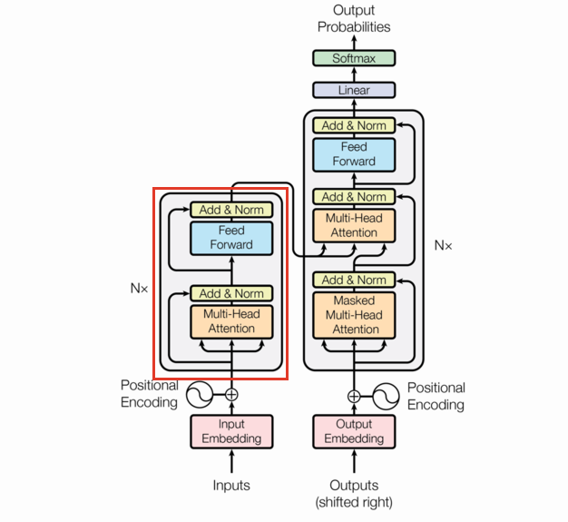
The Encoder is a combination of the various layers we’ve already built up along with several EncoderLayers (which are themselves just combinations of previously defined layers). This section is going to be short.
Note the EncoderLayer takes one argument (neglecting the mask) and feeds that one argument as the query, key, and value in the Multi-Head Attention layer. This can be seen by following the arrows in the diagram.
class EncoderLayer(nn.Module):
    hidden_dim: int
    n_heads: int
    size_per_head: int
    attn_dropout: float
    fc_dropout: float

    def setup(self):
        self.attn = MultiHeadAttention(n_heads=self.n_heads,
                                       size_per_head=self.size_per_head,
                                       attn_dropout=self.attn_dropout,
                                       fc_dropout=self.fc_dropout)
        self.aan_0 = AddAndNorm()
        self.ff = FeedForward(hidden_dim=self.hidden_dim)
        self.aan_1 = AddAndNorm()

    def __call__(self, X, mask=None, *, training=False):
        X1 = self.attn(X, X, X, mask=mask, training=training)
        X = self.aan_0(X, X1)
        X1 = self.ff(X)
        X = self.aan_1(X, X1)
        return X
Encoder
class Encoder(nn.Module):
    pos_encoding: Callable[[int, int], jnp.array]
    vocab_size: int
    embed_dim: int
    layers: Sequence[EncoderLayer]

    @nn.compact
    def __call__(self, X, mask=None, *, training=False):
        B, N = X.shape
        if mask is not None:
            chex.assert_shape(mask, (B, N))
        X = nn.Embed(self.vocab_size, self.embed_dim, name='embed')(X)
        X = X * jnp.sqrt(self.embed_dim)
        # X.shape[-2] is the sequence length
        X = X + self.pos_encoding(X.shape[-2], self.embed_dim)
        for layer in self.layers:
            X = layer(X, mask=mask, training=training)
        return X
There are quite a few parameters, but with some still pathologically small numbers, we get an astronomical $47,670$ parameters!
def layer_fn():
    return EncoderLayer(hidden_dim=13,
                        attn_dropout=0.1,
                        fc_dropout=0.1,
                        n_heads=7,
                        size_per_head=17)
mdl = Encoder(pos_encoding=sin_pos_enc, vocab_size=len(vocab),
              embed_dim=2 * 3 * 5,
              layers=[layer_fn() for _ in range(3)])
batch = strs2ids('hey', 'there', 'ma', 'dood')
mask = (batch == vocab['<pad>'])
params = mdl.init(key, batch)
num_params(params['params'])
47670
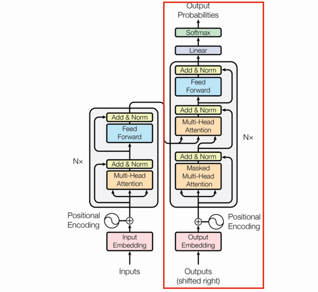
Decoder
The decoder generates new sequences given some input state sequence (maybe the output of the Encoder). You build up a sequence by iteratively asking the model for the next token until either some stop criteria or you get a token signifying the end of the sequence (we’re using "<pad>" for this). This iterative approach cannot be parallelized efficiently.
Causal masking
Transformers can train on full sequences without the recursion, but it requires the clever so called, causal masking. When computing gradients, it’s important that output token $i$ cannot attend to any later output token $i+k$ as they won’t be available in production.
def causal_mask(shape):
    return jnp.triu(jnp.ones(shape, dtype=jnp.bool_), k=1)

causal_mask((1, 5, 5))
Array([[[False,  True,  True,  True,  True],
        [False, False,  True,  True,  True],
        [False, False, False,  True,  True],
        [False, False, False, False,  True],
        [False, False, False, False, False]]], dtype=bool)
DecoderLayer
One thing to note: decoder only transformer layers remove the cross attention layer (the middle attention).
class DecoderLayer(nn.Module):
    hidden_dim: int
    n_heads: int
    size_per_head: int
    attn_dropout: float
    fc_dropout: float

    @nn.compact
    def __call__(self, X_enc, X_dec, enc_mask, dec_mask, *, training=False):

        def attn(q, kv, mask, training, name):
            mdl = MultiHeadAttention(n_heads=self.n_heads,
                                     size_per_head=self.size_per_head,
                                     attn_dropout=self.attn_dropout,
                                     fc_dropout=self.fc_dropout,
                                     name=f'{name}_attn')
            out = mdl(q, kv, kv, mask=mask, training=training)
            aan = AddAndNorm(name=f'{name}_addnorm')
            return aan(q, out)
        X_dec = attn(X_dec, X_dec, dec_mask, training, 'self')
        X_dec = attn(X_dec, X_enc, enc_mask, training, 'src')
        X1 = FeedForward(hidden_dim=self.hidden_dim)(X_dec)
        X_dec = AddAndNorm()(X_dec, X1)
        return X_dec
class Decoder(nn.Module):
    pos_encoding: Callable[[int, int], jnp.array]
    vocab_size: int
    embed_dim: int
    layers: Sequence[DecoderLayer]

    @nn.compact
    def __call__(self, X_enc, X_dec, enc_mask, *, training=False):
        B, N = X_dec.shape[:2]
        dec_mask = causal_mask((1, N, N))
        X_dec = nn.Embed(self.vocab_size, self.embed_dim, name='embed')(X_dec)
        X_dec = X_dec * jnp.sqrt(self.embed_dim)
        # X.shape[-2] is the sequence length
        X_dec = X_dec + self.pos_encoding(X_dec.shape[-2], self.embed_dim)
        for layer in self.layers:
            X_dec = layer(X_enc, X_dec, enc_mask, dec_mask, training=training)
        X_dec = nn.Dense(self.vocab_size, name='final')(X_dec)
        return X_dec
Checking the size of these models using the same hyperparameters as we did with the Encoder… 91 thousand parameters!
def layer_fn():
    return DecoderLayer(hidden_dim=13,
                        attn_dropout=0.1,
                        fc_dropout=0.1,
                        n_heads=7,
                        size_per_head=17)
mdl = Decoder(pos_encoding=sin_pos_enc,
              vocab_size=len(vocab),
              embed_dim=2 * 3 * 5,
              layers=[layer_fn() for _ in range(3)])
batch = strs2ids('hey', 'there', 'ma', 'dood')
kv = strs2ids('i', 'really', 'enjoy', 'algorithms')
enc_mask = (kv == vocab['<pad>'])
kv = nn.one_hot(kv, len(vocab))
params = mdl.init(key, kv, batch, enc_mask)
print(f'{num_params(params) = }')
del layer_fn, mdl, batch, kv, enc_mask, params
num_params(params) = 91291
Flavors
Transformers come in three main flavors.
Encoder-only
- These take in a sequence and output state features.
- It’s mostly useful for tasks like text classification, sentiment analysis, stuff like that.
- One notable example is Google’s bert.
Decoder-only
Decoder only transformers remove the middle multi-head attention (the cross-attention) layer as there is nothing to cross with.
- These are called generative models.
- They take a static state and generate a sequence iteratively.
- Mostly useful for text (media) generation1.
- One notable example: GPT.
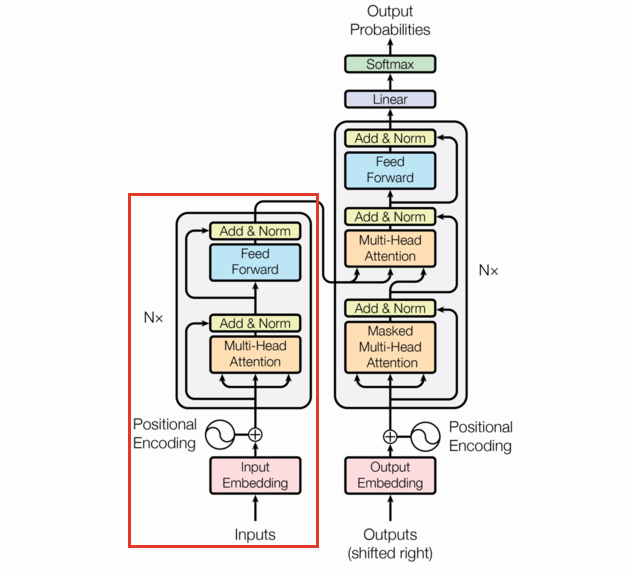
Encoder-decoder
- These models are officially just this diagram.
- They’re of a class of models called seq2seq models.
- They take sequence inputs, generate some state features (via the encoder), and generate a sequence output (via the decoder).
- As such, they’re typically used as translation models.
And as we’ll see in a minute, they can be used to compute rot13 encryption!
class EncoderDecoderTransformer(nn.Module):
    pos_encoding: Callable[[int, int], jnp.array]
    in_vocab_size: int
    out_vocab_size: int
    embed_dim: int
    n_layers: int
    hidden_dim: int
    attn_dropout: float
    fc_dropout: float
    n_heads: int
    size_per_head: int

    def setup(self):
        self.encoder = Encoder(
            pos_encoding=self.pos_encoding,
            vocab_size=self.in_vocab_size,
            embed_dim=self.embed_dim,
            layers=[EncoderLayer(hidden_dim=self.hidden_dim,
                                 attn_dropout=self.attn_dropout,
                                 fc_dropout=self.fc_dropout,
                                 n_heads=self.n_heads,
                                 size_per_head=self.size_per_head,
                                 name=f'encoder_{i}')
                    for i in range(self.n_layers)])
        self.decoder = Decoder(
            pos_encoding=self.pos_encoding,
            vocab_size=self.out_vocab_size,
            embed_dim=self.embed_dim,
            layers=[DecoderLayer(hidden_dim=self.hidden_dim,
                                 attn_dropout=self.attn_dropout,
                                 fc_dropout=self.fc_dropout,
                                 n_heads=self.n_heads,
                                 size_per_head=self.size_per_head,
                                 name=f'decoder_{i}')
                    for i in range(self.n_layers)])

    def __call__(self, X, Y, source_mask, *, training=False):
        # required for dot product attention
        chex.assert_equal(self.encoder.embed_dim, self.decoder.embed_dim)
        encodings = self.encoder(X, source_mask, training=training)
        self.sow('intermediates', 'encodings', encodings)
        return self.decoder(encodings, Y, source_mask, training=training)
A tiny EncoderDecoder model has over 140 thousand parameters. And we’re not even trying yet.
mdl = EncoderDecoderTransformer(
    pos_encoding=sin_pos_enc,
    in_vocab_size=len(vocab),
    out_vocab_size=len(vocab),
    embed_dim=2 * 3 * 5,
    n_layers=3,
    hidden_dim=13,
    attn_dropout=0.1,
    fc_dropout=0.1,
    n_heads=7,
    size_per_head=3
)
X = strs2ids('hey', 'there', 'ma', 'dood')
y = strs2ids('i', 'really', 'enjoy', 'algorithms')
mask = (X == vocab['<pad>'])
params = mdl.init(key, X, y, mask)
print(f'{num_params(params) = }')
del mdl, X, y, mask, params
num_params(params) = 31903
Example
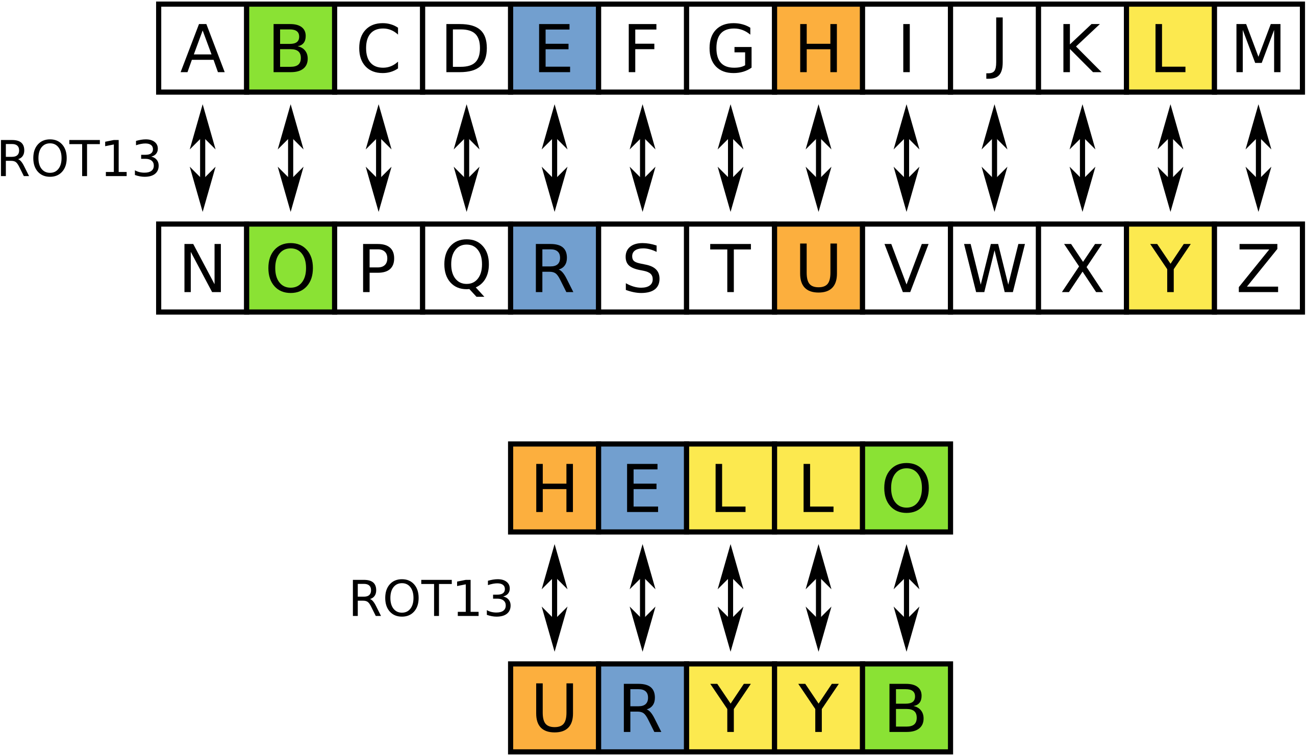
Rot13
We’re going to train our transformer to encrypt words via rot13. Rot13 is an old-school encryption algorithm where each character is shifted by 13 characters (see below).
Training a transformer to do rot13 is a bit like using a chainsaw to give an injection but it’s simple so it’s well suited to purpose.
Since there are 26 letters in the English alphabet, rot13 is its own inverse! That means if you encode a message with rot13 twice, you get back the original message.
def rot13(input_string):
    return ''.join([chr(((vocab[x] + 13) % 26) + 97) for x in input_string])

a = 'asdfqwerz'
print(a, '=>', rot13(a), '=>', rot13(rot13(a)))
del a
asdfqwerz => nfqsdjrem => asdfqwerz
Let’s write our data generator.
def get_data(key):
    k0, k1 = jran.split(key, 2)
    max_len = 15
    X = jran.randint(k0, (50, max_len), 0, len(vocab) - 2)
    mask = jnp.stack([jnp.arange(max_len) >= i for i in jran.randint(k1, (50,), 1, max_len)])
    X = X * (1 - mask) + (mask * vocab['<pad>'])
    Y = ((X + 13) % (len(vocab) - 2))  # cheap version of rot13 at the encoded level
    Y = (1 - mask) * Y + mask * vocab['<pad>']
    Ys = (
        jnp.ones_like(Y, dtype=jnp.int32)
        .at[:, 1:].set(Y[:, :-1])
        .at[:, 0].set(vocab['<start>'])
    )
    return (X, Ys, mask.astype(jnp.float32)), Y
mdl = EncoderDecoderTransformer(pos_encoding=sin_pos_enc,
                                in_vocab_size=len(vocab),
                                out_vocab_size=len(vocab),
                                embed_dim=8,
                                n_layers=1,
                                hidden_dim=5,
                                attn_dropout=0.0,
                                fc_dropout=0.0,
                                n_heads=7,
                                size_per_head=5)

opt = optax.chain(
    optax.clip_by_global_norm(1),
    optax.sgd(
        learning_rate=optax.warmup_exponential_decay_schedule(
            init_value=0.5, peak_value=0.8, warmup_steps=100,
            transition_steps=200, decay_rate=0.5,
            transition_begin=100, staircase=False, end_value=1e-3
        )
    )
)

params = mdl.init(key, *get_data(key)[0])
print('num_params: ', num_params(params))
opt_state = opt.init(params)
num_params: 4665
One nice thing about jax is that you don’t compile a model, you compile the whole training loop (which, in our case includes data generation).
@jax.jit
def train_step(params, opt_state, step, key):
    """Train for a single step."""
    k0, k1 = jran.split(jran.fold_in(key, step))
    args, y = get_data(k0)

    @jax.grad
    def grad_fn(params):
        logits = mdl.apply(params, *args,
                           training=True, rngs={'dropout': k1})
        loss = optax.softmax_cross_entropy_with_integer_labels(
            logits, y
        ).mean()
        return loss
    grads = grad_fn(params)
    updates, opt_state = opt.update(
        grads, opt_state, params)
    params = optax.apply_updates(params, updates)
    return params, opt_state
We’ll the 10,000 train steps (which takes about 3 minutes on my laptop)…
for step in tqdm(range(10_000)):
    params, opt_params = train_step(params, opt_state, step, key)
Now let’s run the test.
X = strs2ids('hey', 'there', 'ma', 'dood')
start = jnp.array([[vocab['<start>']]] * X.shape[0], dtype=jnp.int32)
Y = start
while (Y[:, -1] != vocab['<pad>']).any():
    Y = jnp.argmax(mdl.apply(params, X, jnp.concatenate([start, Y], axis=-1), X == vocab['<pad>']), axis=-1)
ids2strs(list(Y))
['url', 'gurer', 'zn', 'qbbq']
[rot13(x) for x in ids2strs(list(Y))]
['hey', 'there', 'ma', 'dood']
And that’s all folks! You can now transform with the best of ‘em!
-
This fact is very quickly becoming outdated. ↩
