$$\text{???} = (MC)^2$$

Background

What if we know the relative likelihood, but want the probability distribution?

$$\mathbb{P}(X=x) = \frac{f(x)}{\int_{-\infty}^\infty f(x)dx}$$

But what if $\int f(x)dx$ is hard, or you can't sample from $f$ directly?

This is the problem we will be trying to solve.

First approach

If space if bounded (integral is between $a,b$) we can use Monte Carlo to estimate $\int\limits_a^b f(x)dx$

• Pick $\alpha \in (a,b)$
• Compute $f(\alpha)/(b-a)$
• Repeat as necessary
• Compute the expected value of the computed values

What if hard?

What if we can't sample from $f(x)$ but can only determine likelihood ratios?

$$\frac{f(x)}{f(y)}$$

Markov Chain Monte Carlo

The obligatory basics

A Markov Chain is a stochastic process (a collection of indexed random variables) such that $\mathbb{P}(X_n=x|X_0,X_1,...,X_{n-1}) = \mathbb{P}(X_n=x|X_{n-1})$.

In other words, the conditional probabilities only depend on the last state, not on any deeper history.

We call the set of all possible values of $X_i$ the state space and denote it by, $\chi$.

Transition Matrix

Let $p_{ij} = \mathbb{P}(X_1 = j | X_0 = i)$. We call the matrix $(p_{ij})$ the Transition Matrix of $X$ and denote it $P$.

Let $\mu_n = \left(\mathbb{P}(X_n=0), \mathbb{P}(X_n=1),..., \mathbb{P}(X_n=l)\right)$ be the row vector corresponding to the "probabilities" of being at each state at the $n$th point in time (iteration).

Claim: $\mu_{i+1} = \mu_0P^{i+1}$

$$\begin{align*} (\mu_0 P)_j =& \sum\limits_{i=1}^l\mu_0(i)p_{ij}\\ =&\sum\limits_{i=1}^l\mathbb{P}(X_0=i)\mathbb{P}(X_1=j | X_0=i)\\ =&\mathbb{P}(X_1 = j)\\ =&\mu_1(j) \end{align*}$$

So: $\mu_1 = \mu_0P$.

Stationary Distributions

We say that a distribution $\pi$ is stationary if

$$\begin{gather*}\pi P = \pi\end{gather*}$$

Limiting Distribution?

Main Theorem:

An irreducible, ergotic Markov Chain $\{X_n\}$ has a unique stationary distribution, $\pi$. The limiting distribution exists and is equal to $\pi$. And furthermore, if $g$ is any bounded function, then with probability 1:

$$\lim\limits_{N\to\infty}\frac{1}{N}\sum\limits_{n=1}^Ng(X_n) \rightarrow E_\pi(g)$$

Random-Walk-Metropolis - Hastings:

Let $f(x)$ be the relative likelihood function of our desired distribution.

$q(y|x)$ known distribution easily sampled from (generally taken to be $N(x,b^2)$)

1) Given $X_0,X_1,...,X_i$, pick $Y \sim q(y|X_i)$

2) Compute $r(X_i,Y) = \min\left(\frac{f(Y)q(X_i|Y)}{f(X_i)q(Y|X_i)}, 1\right)$

3) Pick $a \sim U(0,1)$

4) Set $X_{i+1} = \begin{cases} Y & \text{if } a < r \\ X_i & \text{otherwise}\end{cases}$

The Confidence Builder:

We would like to sample from and obtain a histogram of the Cauchy distribution:

$$f(x) = \frac{1}{\pi}\frac{1}{1+x^2}$$

$$\begin{align*} q_{01} \sim& N(x,0.1)\\ q_1 \sim& N(x,1)\\ q_{10} \sim& N(x,10)\end{align*}$$

Note: Since $q$ is symmetric, $q(x|y) = q(y|x)$!

def metropolis_hastings(f, q, initial_state, num_iters):
    MC = []
    X_i = initial_state
    for i in range(int(num_iters)):
        Y = q(X_i)
        r = min(f(Y)/f(X_i), 1)
        a = np.random.uniform()
        if a < r:
            X_i = Y
        MC.append(X_i)
    return MC

def cauchy_dist(x):
    return 1/(np.pi*(1 + x**2))
def q(scale):
    return lambda x: np.random.normal(loc=x, scale=scale)

from scipy.stats import cauchy
CauchyInterval = np.linspace(cauchy.ppf(0.01),
                             cauchy.ppf(0.99),
                             100);

std01 = metropolis_hastings(cauchy_dist, q(0.1), 0, 1000)
tmpHist = plt.hist(std01, bins=20, normed=True);
tmpLnSp = np.linspace(min(tmpHist[1]),
                      max(tmpHist[1]),100)
plt.plot(tmpLnSp, cauchy.pdf(tmpLnSp), 'r-')
plt.show();

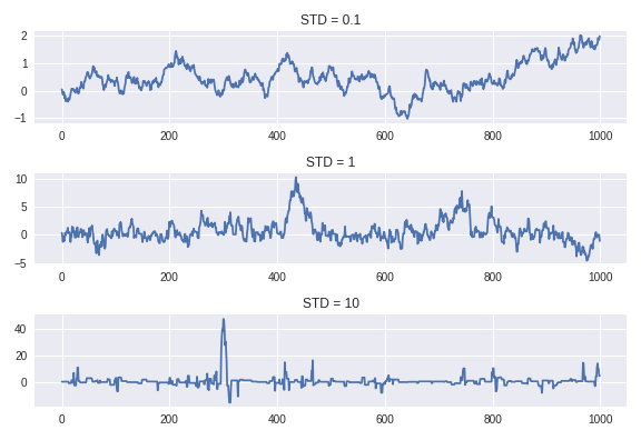
Estimation:

$$q(y|x) \sim N(0,b^2)$$

Another Aspect

How is this happening???

A property called detailed balance, which means, $$\pi_ip_{ij} = p_{ji}\pi_j$$

or in the continuous case: $$f(x)P_{xy} = f(y)P_{yx}$$

But we don't need to go over that... Unless you wanna...

Proof?

Let $f$ be the desired distribution (in our example, it was the Cauchy Distribution), and let $q(y|x)$ be the distribution we draw from.

First we'll show that detailed balance implies $\pi$ (or $f$ if continuous) is the stable distribution!

Let $\pi_ip_{ij} = \pi_jp_{ji}$ for discrete or for continuous $f(i)P_{ij}=P_{ji}f(j)$

$$\begin{align*} (\pi P)_i =& \sum\limits_j\pi_jP_{ji} & (fP)(x)=&\int f(y)p(x|y)dy\\ =&\sum\limits_j\pi_iP_{ij} & =& \int f(x)p(y|x)dy\\ =&\pi_i\sum\limits_jP_{ij} & =& f(x)\int p(y|x)dy\\ =&\pi_i & =& f(x) \end{align*}$$

Now we'll show that our MCMC has the detailed balance property.

WLOG: Assume $f(x)q(x|y) > f(y)q(y|x)$.

Note: $r(x,y) = \frac{f(y)q(x|y)}{f(x)q(y|x)}$, and $r(y,x) = 1$.

Then,

$$\begin{align*} \pi_xp_{xy} =& f(x)p(x\rightarrow y) & \pi_yp_{yx} =& f(y)p(y\rightarrow x)\\ =& f(x)\left[q(y|x)\cdot r(x,y)\right] & =&f(y)\left[q(x|y)\cdot r(y,x)\right]\\ =& f(y)q(x|y) & =&f(y)q(x|y) \end{align*}$$

The intuition

We want equal hopportunity:

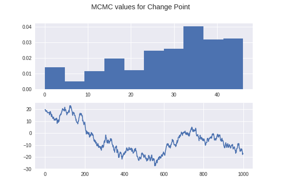
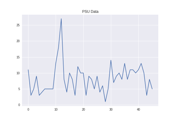
$$f(x)p(x|y) = f(y)p(y|x)$$

$$r(x,y) = \min\left(\frac{f(y)q(y|x)}{f(x)q(x|y)},1\right)$$

Modeling Change Point Models in Astrostatistics.

$$ \begin{align*} f(k,\theta,\lambda,b_1,b_2 | Y) \alpha& \prod\limits_{i=1}^k\frac{\theta^{Y_i}e^{-\theta}}{Y_i!} \prod\limits_{i=k+1}^n\frac{\lambda^{Y_i}e^{-\lambda}}{Y_i!} \\ &\times\frac{1}{\Gamma(0.5)b_1^{0.5}}\theta^{-0.5}e^{-\theta/b_1} \times\frac{1}{\Gamma(0.5)b_2^{0.5}}\theta^{-0.5}e^{-\theta/b_2}\\ &\times\frac{e^{-1/b_1}}{b_1}\frac{e^{-1/b_2}}{b_2}\times \frac{1}{n} \end{align*} $$

%%bash
if [ ! -f tmp/psu_data.tsv ]
then
wget http://sites.stat.psu.edu/~mharan/MCMCtut/COUP551_rates.dat -O tmp/psu_data.tsv
fi

Potential Issues with RWMetropolis-Hastings:

• Requires $f$ to be defined on all of $\mathbb{R}$
  • So transform as needed
• Curse of dimensionality in tuning parameters

Other forms

• Gibbs Sampling

  • Turn high dimensional sampling into iterative one-dimensional sampling

• Gibbs with Metropolis-Hastings

Bibliography

Summer School in Astrostatistics