Probability using Measure Theory
A mathematically rigorous definition of probability, and some examples therein.
The Traditional Definition:
Consider a set $\Omega$ (called the sample space), and a function $X:\Omega\rightarrow\mathbb{R}$ (called a random variable.
If $\Omega$ is countable (or finite), a function $\mathbb{P}:\Omega\rightarrow\mathbb{R}$ is called a probability distribution if it satisfies the following 2 conditions:
-
For each $x \in \Omega$, $\mathbb{P}(x) \geq 0$
-
If $A_i\cap A_j = \emptyset$, then $\mathbb{P}(\bigcup\limits_0^\infty A_i) = \sum\limits_0^\infty\mathbb{P}(A_i)$
And if $\Omega$ is uncountable, a function $F:\mathbb{R}\rightarrow\mathbb{R}$ is called a probability distribution or a cumulative distribution function if it satisfies the following 3 conditions:
-
For each $a,b\in\mathbb{R}$, $a < b \rightarrow F(a)\leq F(b)$
-
$\lim\limits_{x\to -\infty}F(x) = 0$
-
$\lim\limits_{x\to\infty}F(x) = 1$
The Intuition:
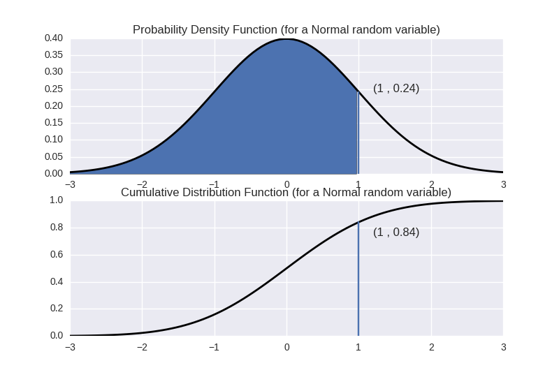
What idea are we even trying to capture with these seemingly disparate definitions for the same thing? Well, with the two cases taken separately it's somewhat obvious, but they don't seem to marry very well. The discrete case is giving us a pointwise estimation of something akin to the proportion of observations that should correspond to a value (in a perfect world). The continuous case is the same thing, but instead of corresponding to that particular value (which doesn't really even make sense in this case), the proportion corresponds to the point in question and everything less than it. The shaded region in the top picture below and the curve in the picture directly below it denote the cumulative density function of a standard normal distribution (don't worry too much about what that means for this post, but if you're doing anything with statistics, you should probably know a bit about that).

Another way to define a continuous probability distribution is through something called a probability density function, which is closer to the discrete case definition of a probability distribution (or probability mass function). A probability density function is a function $f:\mathbb{R}\rightarrow\mathbb{R}_+$ such that $\int_{-\infty}^xf(t)dt = F(x)$. In other words, $\frac{dF}{dX} = f$. This new function has some properties of our discrete case probability function, but lacks some others. On the one hand, they’re both defined pointwise, but on the other, this one can be greater than one in some places – meaning the value of the probability density function isn’t really the probability of an event, but rather (as the name “suggests”) the density therein.
Does it measure up?
Now let’s check out the measure theoretic approach…
Let $\Omega$ be our sample space, $S$ be the $\sigma$-algebra on $\Omega$ (so $S$ is the collection of measurable subsets of $\Omega$), and $\mu:S\to\mathbb{R}$ a measure on that measure space. Let $X:\Omega\rightarrow\mathbb{E}$ be a random variable ($\mathbb{E}$ is generally taken to be $\mathbb{R}$ or $\mathbb{R}^n$). We define the function $\mathbb{P}:\mathcal{P}(\mathbb{E})\rightarrow\mathbb{R}$ (where $\mathcal{P}(\mathbb{E})$ is the powerset of $\mathbb{E}$ – the set of all subsets) such that if $A\subseteq\mathbb{E}$, we have $\mathbb{P}(A)=\mu(X^{-1}(A))$. We call $\mathbb{P}$ a probability distribution if the following conditions hold:
-
$\mu(\Omega) = 1$
-
for each $A\subseteq\mathbb{E}$ we have $X^{-1}(A)\in S$.
Why do this?
Well, right off the bat we have a serious benefit: we no longer have two disparate definitions of our probability distributions. Furthermore, there is the added benefit of having a natural separation of concerns: the measure $\mu$ determines the what we might intuitively consider to be the probability distribution while the random variable is used to encode the aspects of the events that we care about.
To further illustrate this
The Examples
A fair die
All even
Let’s consider a fair die. Our sample space will be ${1,2,3,4,5,6}$. Since our die is fair, we’ll define our measure fairly: for any $x$ in our sample space, $\mu({x}) = \frac{1}{6}$. If we want to know, for instance, what the probability of getting each number is, we could use a very intuitive random variable $X(a) = a$ (so $X(1)=1$, etc.). Then we see that $\mathbb{P}({1}) = \mu({1}) = \frac{1}{6}$, and the rest are found similarly.
Odds and Evens?
What if we want to consider the fair die of yester-paragraph, but we only care if the face of the die shows an odd or an even number? Well, since the actual distribution of the die hasn’t changed, we won’t have to change our measure. Instead we’ll change our random variable to capture just those aspects we care about. In particular, $X(a) = 0$ if $a$ is even, and $X(a) = 1$ if $a$ is odd. We then see $\mathbb{P}(1) = \mu({1,3,5}) = \frac{1}{2}$ and $\mathbb{P}(0) = \mu({2,4,6}) = \frac{1}{2}$
Getting loaded
All even
Now let’s consider the same scenario of wanting to know the probability of getting each number, but now our die is loaded. Being as how we’re changing the distribution itself and not just the aspects we’re choosing to care about, we’re going to want to change the measure this time. For simplicity, let’s consider a kind of degenerate case scenario. Let our measure be: $\mu(A) = 1$ if $1\in A$ and $\mu(A)=0$ if $1\notin A$. Basically, we’re defining our probability to be such that the only possible outcome is a roll of 1. So since we are concerned with the same things we were concerned with last time, we can take that same random variable. We note $\mathbb{P}(1) = 1$ and $\mathbb{P}(a) = 0$ for any $a \neq 1$.
Odds or evens
Try to do this one yourself. I’m going to go get some sleep now. Please feel free to contact me with any questions. I love doing this stuff, so don’t be shy!