 amniskin
$\text{???} = (MC)^2$
Background
What if we know the relative likelihood, but want the probability distribution?
\[\mathbb{P}(X=x) = \frac{f(x)}{\int_{-\infty}^\infty f(x)dx}\]But what if $\int f(x)dx$ is hard, or you can’t sample from $f$ directly?
This is the problem we will be trying to solve.
First approach
If space if bounded (integral is between $a,b$) we can use Monte Carlo to estimate $\int\limits_a^b f(x)dx$
- Pick $\alpha \in (a,b)$
- Compute $f(\alpha)/(b-a)$
- Repeat as necessary
- Compute the expected value of the computed values
The big bag of nope
What if we can’t sample from $f(x)$ but can only determine likelihood ratios?
\[\frac{f(x)}{f(y)}\]Enter Markov Chain Monte Carlo
The obligatory basics
A Markov Chain is a stochastic process (a collection of indexed random variables) such that $\mathbb{P}(X_n=x|X_0,X_1,…,X_{n-1}) = \mathbb{P}(X_n=x|X_{n-1})$.
In other words, the conditional probabilities only depend on the last state, not on any deeper history.
We call the set of all possible values of $X_i$ the state space and denote it by, $\chi$.
Transition Matrix
Let $p_{ij} = \mathbb{P}(X_1 = j | X_0 = i)$. We call the matrix $(p_{ij})$ the Transition Matrix of $X$ and denote it $P$.
Let $\mu_n = \left(\mathbb{P}(X_n=0), \mathbb{P}(X_n=1),…, \mathbb{P}(X_n=l)\right)$ be the row vector corresponding to the “probabilities” of being at each state at the $n$th point in time (iteration).
Claim: $\mu_{i+1} = \mu_0P^{i+1}$
Proof:
if $i = 0$:
\[\begin{align} (\mu\_0 P)\_j =& \sum\limits\_{i=1}^l\mu\_0(i)p\_{ij}\\ =&\sum\limits\_{i=1}^l\mathbb{P}(X\_0=i)\mathbb{P}(X\_1=j \| X\_0=i)\\ =&\mathbb{P}(X\_1 = j)\\ =&\mu\_1(j) \end{align}\]So: $\mu_1 = \mu_0P$
if $i > 0$:
Then, $\mu_{i+1} = \mu_iP = (\mu_0P^i)P = \mu_0P^{i+1}$
Stationary Distributions
We say that a distribution $\pi$ is stationary if
\[\begin{gather}\pi P = \pi\end{gather}\]Main Theorem
An irreducible, ergotic Markov Chain ${X_n}$ has a unique stationary distribution, $\pi$. The limiting distribution exists and is equal to $\pi$. And furthermore, if $g$ is any bounded function, then with probability 1:
\[\lim\limits_{N\to\infty}\frac{1}{N}\sum\limits_{n=1}^Ng(X_n) \rightarrow E_\pi(g)\]This really just means that if our Markov Chain has certain properties (basically just that any state can be gotten to from any other state at any time), then we can sample from this Markov Chain, and it’ll have the same distribution as a generic sample from our desired distribution.
Random-Walk-Metropolis - Hastings:
Let $f(x)$ be the relative likelihood function of our desired distribution.
And $q(y|x_i)$ the known distribution easily sampled from (generally taken to be $N(x_i,b^2)$ )
1) Given $X_0,X_1,…,X_i$, pick $Y \sim q(y|X_i)$
2) Compute $r(X_i,Y) = \min\left(\frac{f(Y)q(X_i|Y)}{f(X_i)q(Y|X_i)}, 1\right)$
3) Pick $a \sim U(0,1)$
4) Set
\[X_{i+1} = \begin{cases} Y & \text{if } a < r \\ X_i & \text{otherwise}\end{cases}\]The Confidence Builder:
We would like to sample from and obtain a histogram of the Cauchy distribution:
\[f(x) = \frac{1}{\pi}\frac{1}{1+x^2}\] \[\begin{align*} q_{01} \sim& N(x,0.1)\\ q_1 \sim& N(x,1)\\ q_{10} \sim& N(x,10)\end{align*}\]Note: Since $q$ is symmetric, $q(x|y) = q(y|x)$.
Pseudocode:
MC = []
X_i = initial_state
for i in range(num_iters):
	Y = q(X_i)
	r = min(f(Y)/f(X_i), 1)
	a = np.random.uniform()
	if a < r:
		X_i = Y
	MC.append(X_i)
Estimation:
\[q(y\|x) \sim N(x,b^2)\]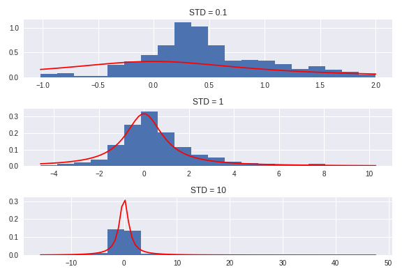
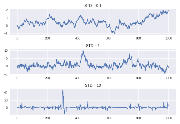
So you can clearly see that the different values of $b$ lead to wildly different distributions, and therefore wildly different approximations of the end distribution. For example, if the standard deviation on our sampling distribution is very small, our prospective transitions won’t venture out very far, and hence the tails of our distribution will be woefully underrepresented. If, on the other hand, the standard deviation is too large, we will often venture our much further than we should, and the we’ll end up with something like a multi-modal distribution. Basically, the prospective transition states will often be too far out to accept, in which case the current state persists, or it will be just close enough to be accepted. What you end up with is far too many samples from the tails and not enough samples from the beafier parts of the distribution.
Choosing the “best” value of $b$ is more of an art than a science, really. This issue will poke its ugly head a little later. But even with that issue, we see clearly that something amazing is happening here.
How is this happening?
A property called detailed balance, which means,
\[\pi_ip_{ij} = p_{ji}\pi_j\]or in the continuous case:
\[f(x)P_{xy} = f(y)P_{yx}\]The intuition
Since what we’re really after is the distribution of the samples and not the order in which they were picked, it’s reasonable to require a notion of (what I’m going to call) equal hopportunity:
\[f(x)p(y\|x) = f(y)p(x\|y)\]In other words, the probability of “hopping” from $x$ to $y$ should be the same as the reverse, because at the end of the day, both of these two scenarios only mean that $x$ and $y$ are in our sample.
If you work out the math therein (as we will do below), you find that this ratio guarantees equal hopportunity.
\[r(x,y) = \min\left(\frac{f(y)q(x\|y)}{f(x)q(y\|x)},1\right)\]Let’s prove it!
To reiterate, the claim was that this detailed balance property ( $f(x)P_{xy} = P_{yx}f(y)$ ) guarantees that our likelihood function $f$ is the stable distribution for our Markov Chain.
Let $f$ be the desired distribution (in our example, it was the Cauchy Distribution), and let $q(y|x)$ be the distribution we draw from.
First we’ll show that detailed balance implies $\pi$ (or $f$ if the distribution is continuous) is the stable distribution!
Let $\pi_ip_{ij} = \pi_jp_{ji}$ for discrete or for continuous $f(i)P_{ij}=P_{ji}f(j)$
\[\begin{align*} (\pi P)\_i =& \sum\limits\_j\pi\_jP\_{ji} & (fP)(x)=&\int f(y)p(x\|y)dy\\ =&\sum\limits\_j\pi\_iP\_{ij} & =& \int f(x)p(y\|x)dy\\ =&\pi\_i\sum\limits\_jP\_{ij} & =& f(x)\int p(y\|x)dy\\ =&\pi\_i & =& f(x) \end{align*}\]Now we’ll show that the Markov Chain defined by the Metropolis-Hastings algorithm has the detailed balance property (and hence $f$ is the stable distribution).
Without any loss of generality, we’ll assume $f(x)q(y|x) > f(y)q(x|y)$ (if this is not the case, the proof will follow the same with just symbolic changes).
Note: Since $f(x)q(y|x) > f(y)q(x|y)$, we know, $r(x,y) = \frac{f(y)q(x|y)}{f(x)q(y|x)}$, and $r(y,x) = 1$.
Then,
\[\begin{align*} \pi_xp_{xy} =& f(x)\mathbb{P}(X_1=y\|X_0=x) & \pi_yp_{yx} =& f(y)\mathbb{P}(X_1=x\|X_0=y)\\ =& f(x)\left[q(y\|x)\cdot r(x,y)\right] & =&f(y)\left[q(x\|y)\cdot r(y,x)\right]\\ =& f(x)\left[q(y\|x)\cdot \frac{f(y)q(x\|y)}{f(x)q(y\|x)}\right] & =&f(y)\left[q(x\|y)\cdot 1\right]\\ =& f(y)q(x\|y) & =&f(y)q(x\|y) \end{align*}\]Modeling Change Point Models in Astrostatistics.
This was taken from a Penn State statistics summer program website located at stat.psu.edu. A detailed walk-through of the process PSU took with this project can be found at that site. The data is a time series of light emission recorded and aggregated over periods of 10000 seconds (just under 3 hours). A plot of the time series can be seen below for your convenience.
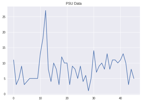
The idea (with this data) is that the emissions can be modeled by two Poisson distributions and a change point. The data will be modeled by the first Poisson until the change point, and then it switches to the second Poisson.
So we start out with a multi-parameter model, and through some Bayesian inference you arrive at a pretty nasty looking posterior distribution. You’d like to sample this distribution to obtain, say, the mean $k$ (change point) value along with a 95% confidence interval. Since you need that confidence interval, standard optimization methods won’t suffice: we’d need the distribution of $k$s. For this, we can use MCMC!
The posterior distribution we would like to sample from is this:
\[\begin{align*} f(k,\theta,\lambda,b_1,b_2 \| Y) \alpha& \prod\limits_{i=1}^k\frac{\theta^{Y_i}e^{-\theta}}{Y_i!} \prod\limits_{i=k+1}^n\frac{\lambda^{Y_i}e^{-\lambda}}{Y_i!} \\ &\times\frac{1}{\Gamma(0.5)b_1^{0.5}}\theta^{-0.5}e^{-\theta/b_1} \times\frac{1}{\Gamma(0.5)b_2^{0.5}}\theta^{-0.5}e^{-\theta/b_2}\\ &\times\frac{e^{-1/b_1}}{b_1}\frac{e^{-1/b_2}}{b_2}\times \frac{1}{n} \end{align*}\]This distribution is pretty gnarly and since I don’t really know how to sample from this (beyond a blind search), we would like to use MCMC. Metropolis-Hastings (at least how we’ve discussed it) clearly doesn’t work here because this is multidimensional. For that we introduce another MCMC algorithm: Gibbs Sampling.
Gibbs Sampling
The basic pseudocode is this:
X = initial_X
Y = initial_Y
...
Z = initial_Z
MC = [(X,Y,...,Z)]
for _ in range(num_iters):
	// for each variable we compute
	X ~ q_X(x|X,Y,...,Z)
	// We do this for X, Y, ..., Z in turn
We can combine Gibbs with Metropolis quite easily:
X = initial_X
Y = initial_Y
...
Z = initial_Z
MC = [(X,Y,...,Z)]
for _ in range(num_iters):
	// for each variable we compute
	prospect ~ q_X(x|X,Y,...,Z)
	r = min(f(prospect)/f(X), 1)
	a ~ uniform(0,1)
	if a < r:
		X = prospect
	// We do this for X, Y, ..., Z in turn
So, basically, you update one at a time.
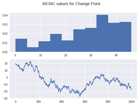
Using this algorithm, we can analyze the data from the PSU website we mentioned above. In fact we did that very thing. Below you’ll find some graphs depicting the distribution of $k$ values.
Summary
- Random-Walk-Metropolis-Hastings
- Can be used to sample difficult univariate distributions relatively easily
- Have to tune the sampling parameter
- Curse of dimensionality in tuning parameters
- Requires $f$ to be defined on all of $\mathbb{R}$
- Transform as needed
- Can be used to sample difficult univariate distributions relatively easily
- Gibbs Sampling
- Turn high dimensional sampling into iterative one-dimensional sampling
- Gibbs with Metropolis-Hastings
- Lovely