Linear Regression -- The Basics

The basics

Yeah. It’s not a good sign if I’m starting out already repeating myself. But that’s how things seem to be with linear regression, so I guess it’s fitting. It seems like every day one of my professors will talk about linear regression, and it’s not due to laziness or lack of coordination. Indeed, it’s an intentional part of the curriculum here at New College of Florida because of how ubiquitous linear regression is. Not only is it an extremely simple yet expressive formulation, it’s also the theoretical basis of a whole slew of other tactics. Let’s just get right into it, shall we?

Linear Regression:

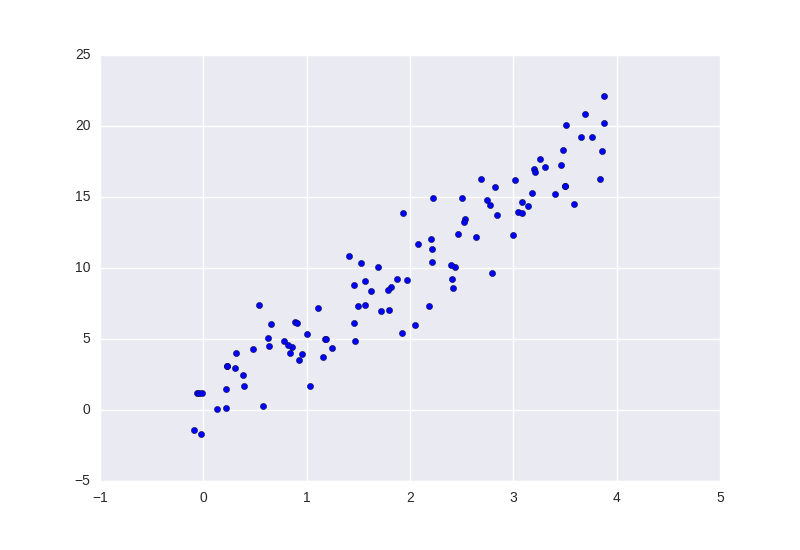
Let’s say you have some data from the real world (and hence riddled with real-world error). A basic example for us to start with is this one:

There’s clearly a linear trend there, but how do we pick which linear trend would be the best? Well, one thing we could do is pick the line that has the least amount of error from the prediction to the actual data-point. To do that, we have to say what we mean by “least amount of error”. For this post, we’ll calculate that error by squaring the difference between the predicted value and the actual value for every point in our data set, then averaging those values. This standard is called the Mean-Squared-Error (MSE). We can write the MSE as:

\[\frac{1}{N}\sum\limits_{i=1}^N\left(\hat Y_i - Y_i\right)^2\]

where $\hat Y_i$ is our predicted value of $Y_i$ for a give $X_i$. Being as how we want a linear model (for simplicity and extensibility), we can write the above equation as,

\[\sum\limits_{i=1}^N\left(\alpha + \beta X_i - Y_i\right)^2\]

for some $\alpha, \beta$ that we don’t yet know. But since we want to minimize that error, we can take some derivatives and solve for $\alpha, \beta$! Let’s go ahead and do that! We want to minimize

\[\sum\limits_{i=1}^N\left(\alpha + \beta X_i - Y_i\right)^2\]

We can start by finding the $\hat\alpha$ such that, $\frac{d}{d\alpha}\sum\limits_{i=1}^N\left(\alpha + \beta X_i - Y_i\right)^2 = 0$. And as long as we don’t forget the chain rule, we’ll be alright…

\[\begin{align*} \sum\limits_{i=1}^N2\left(\alpha + \beta X_i - Y_i\right) =& 0\Longrightarrow\\ \sum\limits_{i=1}^N\left(\alpha + \beta X_i - Y_i\right) =& 0 \Longrightarrow\\ N\alpha + N\beta\bar X - N\bar Y =& 0\Longrightarrow\\ \alpha =& \bar Y - \beta\bar X \end{align*}\]

and we’ll find the $\beta$ such that $\frac{d}{d\beta}\sum\limits_{i=1}^N\left(\alpha + \beta X_i - Y_i\right)^2 = 0$

And following a similar pattern we find (sorry for the editing… Wordpress.com isn’t the greatest therein):

\[\begin{align*} \sum\limits_{i=1}^N2X_i\left(\alpha + \beta X_i - Y_i\right) =& 0\Longrightarrow\\ \alpha\sum\limits_{i=1}^NX_i + \beta\sum\limits_{i=1}^N X_i^2 - \sum\limits_{i=1}^NY_iX_i =& 0\Longrightarrow\\ (\bar Y -\beta\bar X)N\bar X + \beta\sum\limits_{i=1}^NX_i^2 - \sum\limits_{i=1}^NY_iX_i =& 0\\ N\bar Y\bar X -N\beta(\bar X)^2 + \beta\sum\limits_{i=1}^NX_i^2 - \sum\limits_{i=1}^NY_iX_i =& 0\\ \beta\left(\sum\limits_{i=1}^NX_i^2 - N(\bar X)^2\right) =& \sum\limits_{i=1}^NY_iX_i - N\bar Y\bar X\\ \beta =& \frac{\sum\limits_{i=1}^NY_iX_i - N\bar Y\bar X}{\sum\limits_{i=1}^NX_i^2 - N(\bar X)^2} \end{align*}\]

But note:

\[\text{VAR}(X) = \frac{1}{N}\sum\limits_{i=1}^NX_i^2 - (\bar X)^2\]

So,

\[N\cdot\text{VAR}(X) = \sum\limits_{i=1}^NX_i^2 - N(\bar X)^2\]

And: \(\begin{align*} \sum\limits_{i=1}^NY_iX_i - N\bar Y\bar X =& \sum\limits_{i=1}^NY_iX_i - N(\frac{1}{N}\sum\limits_{i=1}^NY_i)\bar X \\ =& \sum\limits_{i=1}^NY_iX_i - \sum\limits_{i=1}^N(Y_i\bar X)\\ =& \sum\limits_{i=1}^NY_i\left(X_i - \bar X\right) \\ =& \sum\limits_{i=1}^NY_i\left(X_i - \bar X\right) - \sum\limits_{i=1}^N\bar Y\left(X_i - \bar X\right) + \sum\limits_{i=1}^N\bar Y\left(X_i - \bar X\right)\\ =& \sum\limits_{i=1}^N\left(Y_i-\bar Y\right)\left(X_i - \bar X\right) + \bar Y\sum\limits_{i=1}^N\left(X_i - \bar X\right)\\ =& \sum\limits_{i=1}^N\left(Y_i-\bar Y\right)\left(X_i - \bar X\right) = N\cdot \text{COV}(X, Y) \end{align*}\)

So,

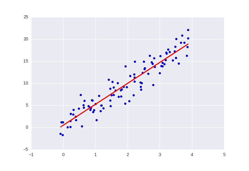
\[\beta = \frac{\text{COV}(X,Y)}{\text{VAR}(X)}\]

And then we can find $\alpha$ by substituting in our approximation of $\beta$. Using those coefficients, we can plot the line below, and as you can see, it really is a good approximation.

Now we have it

Okay, so now we have our line of “best fit”, but what does it mean? Well, it means that this line predicts the data we gave it with the least error. That’s really all it means. And sometimes, as we’ll see later, reading too much into that can really get you into trouble.

But using this model we can now predict other data outside the model. So, for instance, in the model pictured above, if we were to try and predict $Y$ when $X=2$, we wouldn’t do so bad by picking something around 10 for $Y$.

An example, perhaps?

So I feel at this point, it’s probably best to give an example. Let’s say we’re trying to predict stock price given the total market price. Well, in practice this model is used to assess volatility, but that’s neither here nor there. Right now, we’re really only interested in the model itself. But without further ado, I present you with, the CAPM (Capital Asset Pricing Model):

\(r = \alpha + \beta r_m + \epsilon\) (where $\epsilon$ is the error in our predictions).

And you can fit this using historical data or what-have-you. There are a bunch of downsides to fitting it with historical data though, like the fact that data from 3 days ago really doesn’t have much to say about the future anymore. There are plenty of cool things you can do therein, but sadly, those are out of the scope of this post.

For now, we move on to

Multiple Regression

What is this anyway?

Well, multiple regression is really just a new name for the same thing: how do we fit a linear model to our data given some set of predictors and a single response variable? The only difference is that this time our linear model doesn’t have to be one dimensional. Let’s get right into it, shall we?

So let’s say you have $k$ many predictors arranged in a vector (in other words, our predictor is a vector in $\mathbb{R}^n$). Well, I wonder if a similar formula would work… Let’s figure it out…

Firstly, we need to know what a derivative is in $\mathbb{R}^n$. Well, if $f:\mathbb{R}^n\to\mathbb{R}^m$ is a differentiable function, then for any $x$ in the domain, $f’(x)$ is the linear map $A: \mathbb{R}^n \to \mathbb{R}^m$ such that $\text{lim}_{h \to 0}\frac{||f(x+h) - f(x) - Ah||}{||h||} = 0$. Basically, $f’(x)$ is the tangent plane.

So, now that we got that out of the way, let’s use it! We want to find the linear function that minimizes the Euclidean norm of the error terms (just like before). But note: the error term is $\epsilon = Y - \hat Y = Y - \alpha -\beta X$, for some vector $\alpha$ and some matrix $\beta$. Now, since it’s easier and it’ll give us the same answer, we’re going to minimize the squared error term instead of just the error term (like we did in the one dimensional version). We’re also going to make one more simplification: That $\alpha=0$. We can do this safely by simply appending (or prepending) a 1 to the rows of our data (thereby creating a constant term). So for the following, assume we’ve done that.

\[\begin{align} \langle\epsilon, \epsilon\rangle =& (Y - X\beta)^T(Y - X\beta) \\ \langle\epsilon, \epsilon\rangle =& (Y^T - \beta^TX^T)(Y - X\beta) \\ \langle\epsilon, \epsilon\rangle =& Y^TY - 2Y^TX\beta + \beta^TX^TX\beta \end{align}\]

So, let’s find the $\beta$ that minimizes that.

\[\begin{align} 0=&\lim\limits_{h\to0}\frac{\|(Y^TY - 2Y^TX(\beta+h) + (\beta+h)^TX^TX(\beta+h)) - (Y^TY - 2Y^TX\beta + \beta^TX^TX\beta) - Ah\|}{\|h\|} \\ 0=&\lim\limits_{h\to0}\frac{\|- 2Y^TXh + 2\beta^TX^TXh + h^TX^TXh - Ah\|}{\|h\|}\\ 0=&\lim\limits_{h\to0}\|- 2Y^TX + 2\beta^TX^TX + h^TX^TX - A\|\frac{\|h\|}{\|h\|}\\ 0=&\lim\limits_{h\to0}\|- 2Y^TX + 2\beta^TX^TX - A\| \end{align}\]

So, now we see that the derivative is $-2Y^TX + 2\beta^TX^TX$ and we want to find where our error is minimized, so we want to set that derivative to zero:

\[\begin{align*} 0=&- 2Y^TX + 2\beta^TX^TX \\ X^TX\beta =& X^TY \\ \beta =& (X^TX)^{-1}X^TY \end{align*}\]

And there we have it. That’s called the normal equation for linear regression.

Maybe next time I’ll post about how we can find these coefficients given some data using gradient descent, or some modification thereof.

Till next time, I hope you enjoyed this post. Please, let me know if something could be clearer or if you have any requests.